Extraction of the wake induction and angle of attack on rotating wind turbine blades from PIV and CFD results

Herráez, Iván; Daniele, Elia; Schepers, J. Gerard

doi:https://doi.org/10.5194/wes-3-1-2018

Articles | Volume 3, issue 1

https://doi.org/10.5194/wes-3-1-2018

Special issue:

Wind Energy Science Conference 2017

https://doi.org/10.5194/wes-3-1-2018

Articles | Volume 3, issue 1

Research article

17 Jan 2018

Research article |

| 17 Jan 2018

Extraction of the wake induction and angle of attack on rotating wind turbine blades from PIV and CFD results

Iván Herráez, Elia Daniele, and J. Gerard Schepers

Abstract

The analysis of wind turbine aerodynamics requires accurate information about the axial and tangential wake induction as well as the local angle of attack along the blades. In this work we present a new method for obtaining them conveniently from the velocity field. We apply the method to the New Mexico particle image velocimetry (PIV) data set and to computational fluid dynamics (CFD) simulations of the same turbine. This allows the comparison of experimental and numerical results of the mentioned quantities on a rotating wind turbine. The presented results open up new possibilities for the validation of numerical rotor models.

Please read the corrigendum first before continuing.

Download & links

Article (PDF, 3055 KB)

Notice on corrigendum
The requested paper has a corresponding corrigendum published. Please read the corrigendum first before downloading the article.
Article (3055 KB)

Corrigendum

Download & links

The requested paper has a corresponding corrigendum published. Please read the corrigendum first before downloading the article.

How to cite.

Received: 22 Sep 2017 – Discussion started: 04 Oct 2017 – Revised: 20 Nov 2017 – Accepted: 29 Nov 2017 – Published: 17 Jan 2018

1 Introduction

The wake induction and the angle of attack (AoA) are crucial quantities for the design and analysis of wind turbines. Several methods have been proposed for their estimation (Hansen et al., 1997; Shen et al., 2009), although their application has been restricted to numerical results (Johansen and Sørensen, 2004; Sørensen et al., 2002). The only exception we are aware of is the work of Yang et al. (2011), who applied the method proposed by Shen et al. (2006) to the experimental data set of the MEXICO turbine. The reason for applying those methods almost exclusively to numerical results is that they usually require more input data than typically available from experiments. Hence, the computation of lift and drag blade characteristics from pressure sensors requires the AoA to be computed beforehand from simulations (Bechmann et al., 2011; Herráez et al., 2014). The experimental blade characteristics are therefore paradoxically influenced by the uncertainties of the simulations. Furthermore, pressure measurements are usually only available for a few radial positions, so that the obtainable spanwise resolution is very coarse (Herráez et al., 2014; Sørensen et al., 2002). In addition, according to our experience many of the available methods are often rather complicated to employ and automatize. Last but not least, existing methods usually require user-defined input parameters such as control points or correction models for the root and tip (Rahimi et al., 2018). This increases the uncertainty of the calculations.

1.1 Scope and outline

In order to address the mentioned issues, this work aims to provide a simple method for obtaining the wake induction and the AoA from the velocity field in the rotor plane. The required flow data can be captured experimentally e.g. by means of particle image velocimetry (PIV) or numerically with computational fluid dynamics (CFD) models. The new method is not only straightforward in its application but also independent from user-defined input parameters. Furthermore, it takes advantage of the high resolution of PIV and CFD results for obtaining detailed spanwise distributions of the quantities searched.

A brief description of the most common methods for the determination of the wake induction and the AoA is presented in Sect. 2.1. The new method is then introduced in Sect. 2.2. Section 3 describes the experimental and numerical data sets used for our calculations. In Sect. 4 the results of applying the proposed method to the mentioned data sets are presented. The conclusions of this work are then summarized in Sect. 5.

2 Determination of the wake induction and the angle of attack

The main challenge for determining the local wake induction and the AoA is to obtain the local velocity in the rotor plane without blade bound circulation influences. Once the local undisturbed velocity components are known, the axial and tangential induction factors (a and a^′, respectively) as well as the AoA are computed as

\begin{array}{l} (1) & a = & 1 - \frac{u_{ax}}{u_{\infty}} \\ (2) & a^{'} = & - \frac{u_{tan}}{ω \cdot r} \\ (3) & A o A = & \arctan (\frac{u_{ax}}{u_{tan}}) - θ, \end{array}

where u_ax and u_tan are, respectively, the rotor plane axial and tangential velocity components free of blade induction influences, u_∞ is the free-stream velocity and θ is the sum of the pitch and local twist angles.

2.1 Available methods

As seen above, the determination of the wake induction and the AoA requires detailed information about the rotor flow without blade induction. A comparison of several methods for obtaining them concluded that three out of four methods were reasonably consistent and reliable (Guntur et al., 2011). In a very recent benchmark study of multiple methods for computing the AoA (including the one presented here), similar results were obtained from all methods except at the tip and root of the blade, where substantial disagreement between some methods was found (Rahimi et al., 2018). A detailed description of all the existing methods is out of the scope of this article, although the reader is referred to Guntur et al. (2011) and Rahimi et al. (2018) for a good overview of the different methods. However, the main ideas behind the most common methods are described in the following:

Inverse blade element momentum (BEM) method. Given the loads along a blade (which can be obtained from experiments or CFD simulations), the BEM theory can be applied as a reverse engineering model for obtaining the wake induction and AoA. A major drawback of this method is that it strongly relies on the basic assumptions of BEM and the corresponding correction models (e.g. for rotational augmentation and tip effects).
Azimuthal averaging technique (AAT) by Hansen et al. (1997). Several equidistant rings upstream and downstream of the rotor plane are used for probing the velocity field at the radial positions of interest. The average velocity of each ring is then calculated. Finally, the velocity in the rotor plane is computed by interpolating the average velocities of all the rings upstream and downstream of the rotor.
Methods proposed by Shen et al. (2006, 2009). For each spanwise position of interest, the velocity field is probed at just one control point of the rotor plane. The blade-induced velocity at that point is computed using the law of Biot–Savart. For this, the local bound circulation of all blades must be computed beforehand. In the first version of the method, the bound circulation is assumed to be a point vortex and only the velocity and surface pressure fields are required for its calculation (Shen et al., 2006). In the second version of the method, the bound circulation is distributed along the airfoil, which makes it more realistic (Shen et al., 2009). In that case, the wall shear stress is also required for accurately computing the distributed bound circulation in regions with flow separation. Once the blade-induced velocity is known, it must be subtracted from the velocity that was previously probed from the control point. As a result, the local velocity free of blade induction influences is obtained.

2.2 New method

In our method, the velocities are directly probed at a location in the rotor plane at which the induction of the blades is counterbalanced and cancelled out. With axial, uniform inflow, this condition is fulfilled at the bisectrix between two consecutive blades (this applies for both two-bladed and three-bladed rotors). This probing location is represented in Fig. 1. Along that line, the flow symmetry causes the downwash of the blade ahead of the bisectrix to counterbalance the upwash of the blade behind it. Hence, the velocities extracted from the rotor plane are just influenced by the wake induction and do not need to be corrected for blade induction influences. The validity of the method is demonstrated analytically in Appendix A.

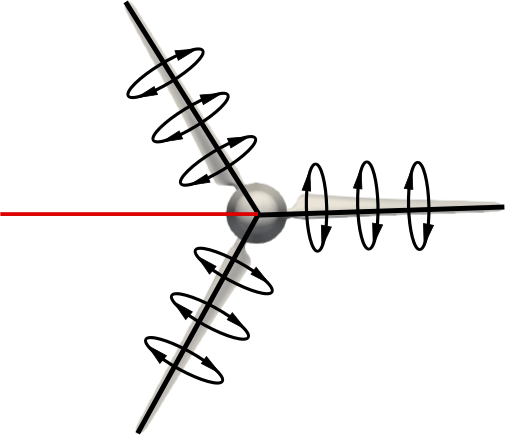
https://www.wind-energ-sci.net/3/1/2018/wes-3-1-2018-f01

Figure 1Schematic representation of the probing location (red line) of the new method for computing the wake induction and the AoA on a rotor operating under axial, uniform inflow. The bound circulation is represented around the blades. Along the red line, the downwash of the blade located at the 11 o'clock position is cancelled out by the upwash of the blade located at the 6 o'clock position. The blade located at the 3 o'clock position does not induce any velocity along the red line. As a result, the velocities obtained along the red line are free of blade induction influences.

Download

The difference between the free-stream velocity and the probed axial velocity corresponds to the axial wake induction. The probed tangential velocity corresponds to the tangential wake induction with opposite sign. Equations (1) and (2) can therefore be directly applied for computing the induction factors. However, it is worth keeping in mind that the non-uniformity of the rotor flow is not only caused by the bound circulation but also by the trailed and shed vorticity. For the cases considered in this work, no shed vorticity needs to be taken into account since the inflow is axial and uniform and the turbine operation is stationary. The trailed vorticity, though, might play a non-negligible role, especially in the tip region. This is the main limitation of the current method since the probing position of the velocity field is located far apart from the blade and consequently the trailed vorticity effects cannot be well captured. The same issue also applies to other well-known and commonly accepted methods, like the AAT, in which the computed velocity values are indeed azimuthal averages. Therefore, we do not expect our method to be less accurate than the AAT, although the mentioned limitation should certainly be kept in mind when extracting the AoA from spanwise positions close to the tip. In order to analyse the severity of this limitation, in Sect. 4 our results are not only compared to the AAT but also to the method proposed by Shen et al. (2006), which has the advantage that it can take better into account the local influence of the trailing vorticity.

In the case of yawed or non-uniform inflow conditions, the new method can still be applied, but it becomes considerably more complex. In that case, the location at which the blade-induced velocities are counterbalanced must be computed by equalizing the induction of all the blades, which must be computed with the law of Biot–Savart. This requires calculating the local bound circulation along each blade beforehand. The simplest way to do this is to compute the line integral of the velocity field along a closed contour located around the blade section and outside the boundary layer.

3 Experimental and numerical data sets

In the following section, the wake induction and the AoA is computed from experimental (PIV) and numerical results of the MEXICO turbine.

PIV windows located just upstream and downstream of the rotor plane are available for the whole blade span (Boorsma and Schepers, 2015). However, a gap of approximately 30 mm exists between both sets of PIV windows, as shown schematically in Fig. 2. Therefore, the data of both measurement sets had to be interpolated in order to obtain the velocities in the rotor plane.

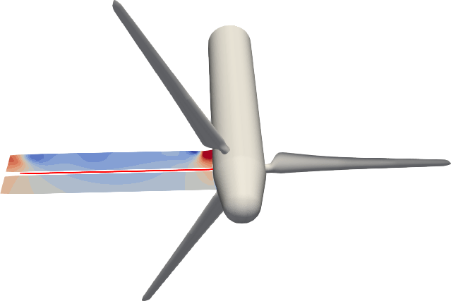
https://www.wind-energ-sci.net/3/1/2018/wes-3-1-2018-f02

Figure 2Schematic representation of the set of PIV windows located at the 3 o'clock position upstream and downstream of the rotor plane. Between both sets of PIV windows there is a gap of approximately 30 mm, in which the bisectrix between the blades (marked in red) is located. The measurements are phase-locked at 60^∘ after blade passage, i.e. when one blade is at the 11 o'clock position (as represented).

Download

The PIV windows were located in a fixed horizontal plane. In this work, we use phase-locked measurements at the azimuth angle 60^∘ after blade passage, corresponding to the bisectrix between two blades, as shown in Fig. 1. The available experimental results for each wind speed are in fact the average of 31 image pairs. More information about the experimental set-up can be found in Boorsma and Schepers (2015).

Axial, uniform inflow conditions with three different wind speeds are considered in this work: 10, 15 and 24 m s⁻¹. At 10 m s⁻¹ the turbine operates in the turbulent wake state, at 15 m s⁻¹ it is at rated conditions and at 24 m s⁻¹ it is stalled. The rotational speed of the rotor is kept constant at 424 rpm, which results in tip speed ratios of λ=10, 6.67 and 4.7, respectively. The pitch angle is $- 2.3^{\circ}$ .

The numerical results used in this work have been extracted from Reynolds-averaged Navier–Stokes simulations of the MEXICO turbine, which were validated against experimental results in Herráez et al. (2014). The reader is referred to that article for a detailed description of the numerical model.

4 Results

The results presented in this section have been computed applying the AAT (see Sect. 2.1) to the CFD simulations of the MEXICO turbine as well as applying the new method introduced in Sect. 2.2 to both the CFD and PIV data of the same turbine. Furthermore, experimental AoA results from the method proposed by Shen et al. (2006) have been extracted from Yang et al. (2011) and are also compared here. The application of the AAT to the experimental results was not possible because it requires more data than available from the experiments.

Figure 3 displays the computed axial induction. When the AAT and the new method are applied to the CFD results, convergent results are obtained in the central region of the blade. However, substantial deviations exist in regions with highly three-dimensional flow, i.e. at the root and the tip. At 10 m s⁻¹ the deviations are stronger at the tip, where a≥0.5. This large induction factor implies that at least the outer part of the rotor operates under the influence of the turbulent wake state.

https://www.wind-energ-sci.net/3/1/2018/wes-3-1-2018-f03

Figure 3Axial induction factor along the rotor radius.

Download

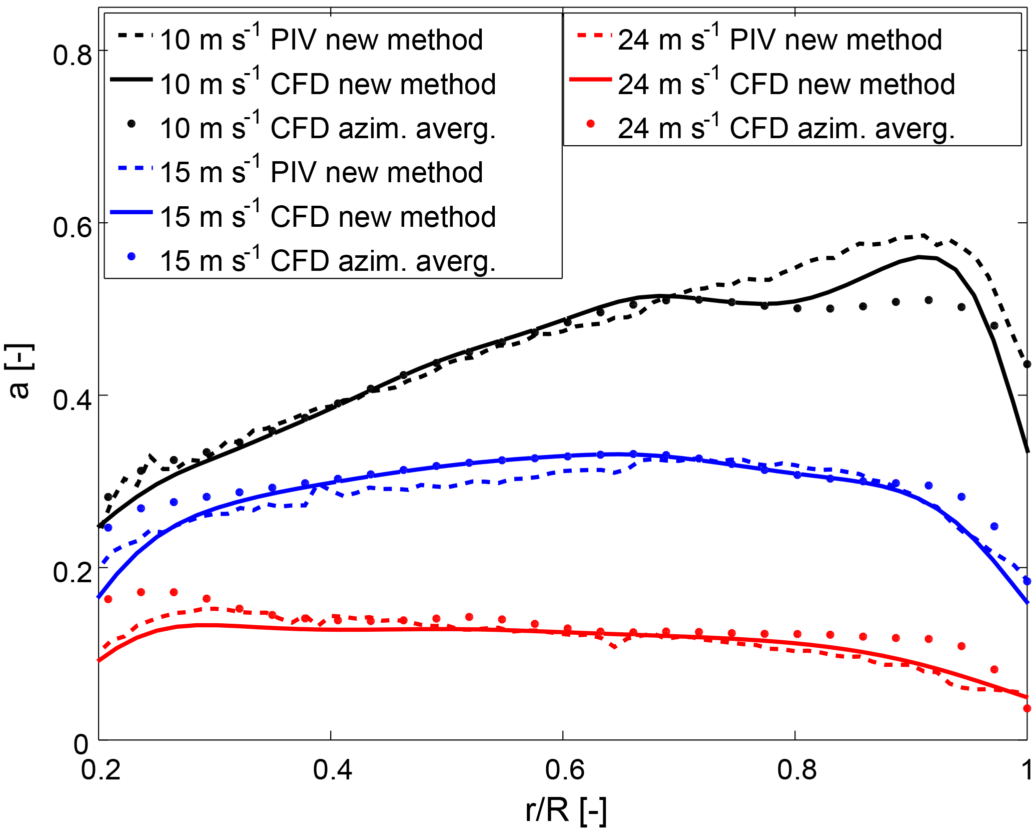
At 15 m s⁻¹ the disagreement is approximately balanced at the tip and the root. At 24 m s⁻¹ the deviations are stronger at the root because of the presence of strong rotational effects (Herráez et al., 2014). It is worth recalling that the AAT method just provides an averaged rotor induction. At the root and the tip, the local induction deviates substantially from the averaged induction as a consequence of the rotor flow non-uniformity, which is attributed to the blade induction and the trailing vorticity influences. The trailing vorticity is not well captured by any of the methods. However, as shown in Sect. 2.2 and demonstrated analytically in Appendix A, the new method correctly accounts for the blade induction influences. This is not the case for AAT; thus, we consider the results obtained with the new method to be more realistic. This interpretation is supported by the results of two different turbines presented in Rahimi et al. (2018), who show that the method proposed by Shen et al. (2006), which presents the advantage of computing the local blade velocities more accurately, is in excellent agreement with our method in the root and tip region, and it also deviates considerably from the AAT.

The results obtained from the CFD and PIV results using the new method compare reasonably well, although clear discrepancies appear in the tip region at 10 m s⁻¹, in the centre of the blade at 15 m s⁻¹ and (to a lower extent) in the root region at 24 m s⁻¹. These discrepancies were already expected because of the complex three-dimensional flows taking place in those regions, as described above. It can therefore be concluded that extracting the wake induction from PIV results opens up new possibilities for the validation of numerical models since until now this was not possible.

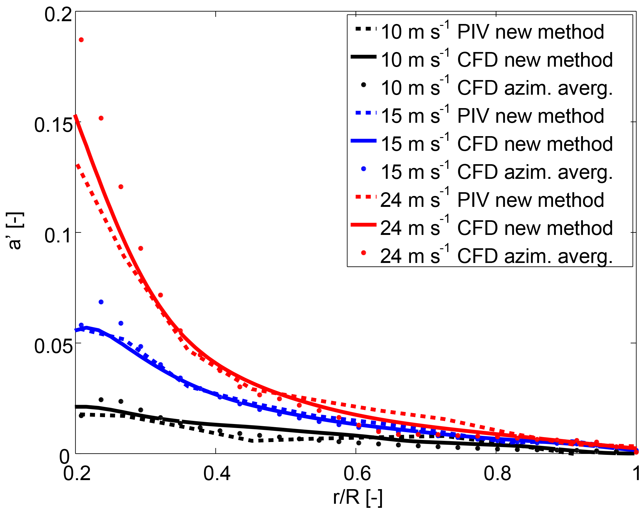
The computed tangential induction factor is displayed in Fig. 4. The results obtained applying the AAT and the new method to the CFD results are in reasonable agreement for outboard positions, where the tangential induction is very low. In the root region, however, substantial discrepancies between both methods appear at 15 and 24 m s⁻¹. The same trend is found when the new method is applied to PIV results. As explained above in relation to the axial induction, this behaviour is attributed to the existence of rotational effects in the root region at stall conditions.

https://www.wind-energ-sci.net/3/1/2018/wes-3-1-2018-f04

Figure 4Tangential induction factor along the rotor radius.

Download

As shown in Fig. 5, the application of the AAT and the new method to the CFD data provides very similar results for most of the blade span in terms of the AoA distribution, with the exception of the root region at 15 m s⁻¹ and (more pronouncedly) at 24 m s⁻¹. The tangential velocity caused by the blade rotation is directly proportional to the radial position and therefore in the root region it is comparatively low. This implies that in the root region deviations in the prediction of the wake induction have a larger impact on the AoA than at outer radial positions. This is the reason why a very good AoA agreement at outboard positions is obtained in spite of the fact that, as shown in Figs. 3 and 4, the wake induction estimations of both methods are not completely consistent. The same observation holds true when comparing the AoA obtained from the application of the new method to the PIV and CFD results. The fact that differences in induction are largely “hidden” in the AoA implies that extracting the AoA from CFD simulations and using it for the calculation of experimental 3-D polars from pressure sensors is a fairly reliable approach when the AoA cannot be directly obtained from experiments.

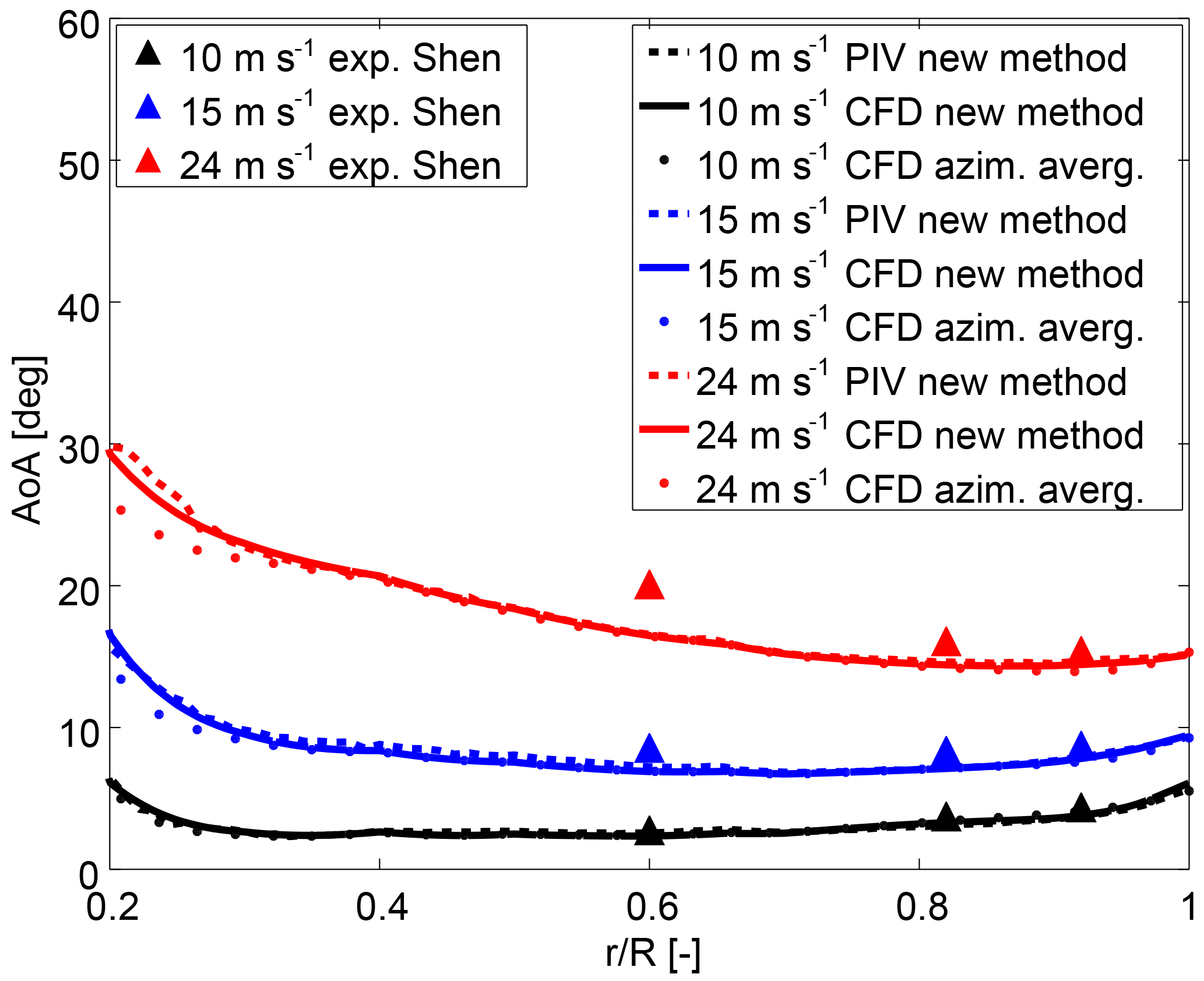
https://www.wind-energ-sci.net/3/1/2018/wes-3-1-2018-f05

Figure 5Angle of attack distribution along the rotor radius comparing three different methods (new method, azimuthal averaging technique and Shen). The results from Shen have been extracted from Yang et al. (2011).

Download

The comparison between the method proposed by Shen et al. (2006) (Yang et al., 2011) and the other methods shows a very good agreement along the whole span for operating conditions involving fully attached flow (i.e. $u_{\infty} = 10 m s^{- 1}$ ). The same happens at the tip ( $r / R = 0.92$ ) for all wind speeds. It is worth remarking that in Yang et al. (2011) several distances between the monitor points and the blade were analysed. The results displayed in Fig. 5 correspond to the smallest distance in order to capture the trailing vorticity effects as accurately as possible Shen et al. (2009). The good agreement between both methods suggests that the tip vortex induction begins to dominate the flow at larger spanwise positions. This is in agreement with Fig. 3.28 in Burton et al. (2011), where it is shown that the induction at the bisectrix between the blades ( $ψ = 60^{\circ}$ ) is representative for the induction at the blade at least up to $r / R = 0.90$ (at $r / R = 0.97$ this does not hold true any more as a consequence of the tip vortex influences).

In Fig. 5, the Shen et al. (2006) method presents a slight deviation in the mid-span region with respect to the other methods for $u_{\infty} = 15 m s^{- 1}$ and a substantial deviation for $u_{\infty} = 24 m s^{- 1}$ . In this context, it is worth recalling that for $u_{\infty} = 15 m s^{- 1}$ , radial flows have been detected in the MEXICO turbine in the mid-span region Herráez et al. (2014), implying flow separation. For $u_{\infty} = 24 m s^{- 1}$ , the radial flows and the flow separation are much more pronounced Herráez et al. (2014). Hence, the use of the Kutta–Joukowski theorem for computing the bound circulation, as it is required in Shen et al. (2006), is not expected to be reliable in that case. The reason for this is that the theorem of Kutta–Joukowski only applies to attached flows. This explains the deviations of the Shen et al. (2006) method from the other results in the mid-span region at separated flow conditions. The same applies to a smaller extent at $r / R = 0.82$ , where the flow is less separated.

5 Conclusions

The method proposed in this work for computing the wake induction and the angle of attack allows the accurate extraction of those quantities from numerical as well as experimental results of the velocity field in the rotor plane. The method is easy to use and automatize for uniform axial inflow. Furthermore, it does not require any user-defined input parameters. The main limitation of the current method, which also applies to other methods, is that it cannot capture the influence of the local trailed and shed vorticities accurately. In principle, this could be an issue at the tip, where the influence of the tip vortex should not be disregarded. However, it has been shown that the method proposed by Shen et al. (2006) (which presents the advantage of capturing the local influences of the trailed and shed vorticities more accurately) provides consistent results with ours up to $r / R = 0.92$ , which suggests that the tip vortex induction begins to dominate the flow at larger spanwise positions. For stall conditions, our method has the advantage over Shen's method that it does not rely on the Kutta–Joukowski theorem, which should only be applied to attached flows.

In the case of yawed or non-uniform inflow, our method can still be used, but it becomes considerably more complicated because of the dependence of the blade bound circulation on the azimuthal blade position.

CFD simulations have been shown to be capable of quite accurately predicting the AoA distribution along the blade span. Therefore, combining the AoA extracted from CFD results with experimental blade pressure measurements can be considered a reliable approach for obtaining realistic lift and drag blade characteristics. Nevertheless, slight deviations with respect to the purely experimental results should be expected in the root region at stall conditions.

The prediction of the wake induction with CFD is much more challenging than the prediction of the AoA, especially in the tip and root regions. This is especially noticeable at operating conditions involving complex, three-dimensional flows.

The direct extraction of the wake induction and the AoA from PIV measurements provides valuable information for the validation of numerical models. Another possible application of the new method is the extraction of 100 % of experimental blade section characteristics (as long as pressure distributions are also available). This, in turn, can contribute to the development or enhancement of engineering correction models for different aerodynamic effects.

Data availability

The employed measurements are available for all participants of the IEA Wind Task 29 MexNext. For more information please contact the third author (schepers@ecn.nl).

Appendix A: Counterbalance of the blade induction at the bisectrix between consecutive blades

The new method proposed in this work for computing the wake induction and the angle of attack on the rotor blades of wind turbines is based on the assumption that for axisymmetric, homogeneous inflow conditions, the induction from the blades bound circulation is counterbalanced at the bisectrix between two blades. In the following, this will be demonstrated for a three-bladed rotor.

At a given point, the velocity induced by the bound circulation of each blade can be computed using the theorem of Biot–Savart:

\begin{matrix} (A1) & V (x, y, z) = \frac{1}{4 π} \int Γ (l) \frac{d l \times r}{| r |^{3}}, \end{matrix}

where

V is the velocity induced in the point $P = (x, y, z)$ .
Γ is the vorticity distribution function of the position (Q) along the blade spanwise direction because of the bound vorticity of a single blade.
l is the coordinate along the blade spanwise direction.
r is the distance between the probe point and the blade element considered.

We introduce two angles:

β is the azimuth angle of the sampling point. It is positive if anticlockwise.
ψ is the azimuth angle of the blade segment. It is positive if anticlockwise.

Expressing the quantities in the Cartesian reference frame we have

\begin{array}{l} (A2) & d l & = (0, d l \sin ψ, d l \cos ψ) \\ (A3) & P & = (0, r \sin β, r \cos β) \\ (A4) & Q & = (0, l \sin ψ, l \cos ψ) \\ (A5) & r & = (0, r \sin β - d l \sin ψ, r \cos β - d l \cos ψ) . \end{array}

The cross product in the Cartesian reference frame results in

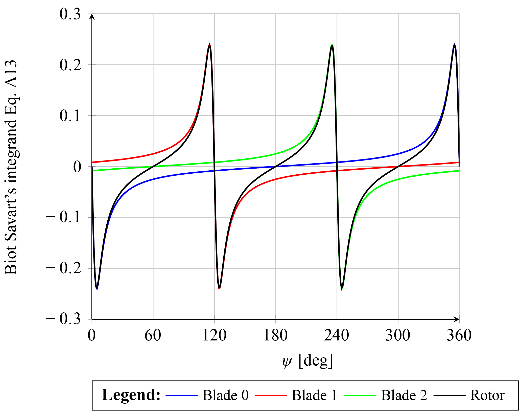
https://www.wind-energ-sci.net/3/1/2018/wes-3-1-2018-f06

Figure A1Biot–Savart's integrand from Eq. (A13) for each blade for a three-bladed rotor (blades located at ψ=0, 120 and 240^∘). The sum of all the blade contributions is shown in black. At the bisectrix between two consecutive blades (ψ=60, 180 and 300^∘), the Biot–Savart's integrand from Eq. (A13) is zero. The blade-induced velocity at those points is consequently also zero.

Download

\begin{array}{l} d l \times r = \\ = & (d l_{y} r_{z} - d l_{z} r_{y}) \hat{i} + \\ (d l_{z} r_{x} - d l_{x} r_{z}) \hat{j} + \\ (d l_{x} r_{y} - d l_{y} r_{x}) \hat{k} \\ = & (d l_{y} r_{z} - d l_{z} r_{y}) \hat{i} + \\ 0 \hat{j} + \\ 0 \hat{k} \\ = & [d l \sin ψ (r \cos β - l \cos ψ) - d l \cos ψ (r \sin β - l \sin ψ)] \hat{i} + \\ 0 \hat{j} + \\ 0 \hat{k} \\ = & d l [r (\cos θ \sin ψ - \sin β \cos ψ) - l (\cos ψ \sin ψ \\ - \cos ψ \sin ψ)] \hat{i} + \\ 0 \hat{j} + \\ 0 \hat{k} \\ = & d l \cdot r (\cos β \sin ψ - \sin β \cos ψ) \hat{i} + \\ 0 \hat{j} + \\ 0 \hat{k} \\ = & d l \cdot r \sin (ψ - β) \hat{i} + \\ 0 \hat{j} + \\ (A6) & 0 \hat{k} . \end{array}

The denominator of the integrand in Eq. (A1) in the Cartesian reference frame results in

\begin{array}{l} | r |^{3} = \\ = & {[(r \sin β - l \sin ψ)^{2} + (r \cos β - l \cos ψ)^{2}]}^{\frac{3}{2}} \\ = & [r^{2} \sin^{2} β + l^{2} \sin^{2} ψ - 2 l r \sin β \sin ψ + r^{2} \cos^{2} β \\ + l^{2} \cos^{2} ψ - 2 l r \cos β \cos ψ]^{\frac{3}{2}} \\ (A7) & = & {[r^{2} + l^{2} - 2 l r \cos (β - ψ)]}^{\frac{3}{2}} . \end{array}

Because of the presence of the sole x component of the induced velocity V, for simplicity we write Eq. (A1) in the Cartesian reference frame as

\begin{matrix} (A8) & u (l, r, β, ψ) = \frac{1}{4 π} \int_{0}^{R} Γ (l) \frac{r \sin (ψ - β)}{{[r^{2} + l^{2} - 2 l r \cos (β - ψ)]}^{\frac{3}{2}}} d l, \end{matrix}

where R is the blade radius. This equation holds for every single blade, $i \in [0, 1, \dots, N - 1]$ , where N is the number of blades for the considered rotor. The difference in azimuthal angle for each blade is simply given by

\begin{matrix} (A9) & Δ ψ = \frac{2 π}{N}, \end{matrix}

being the azimuthal angle of the ith blade given by

\begin{matrix} (A10) & ψ_{i} = ψ_{0} + i Δ ψ . \end{matrix}

Thus, the velocity from the ith blade could be expressed in terms of the 0th blade azimuthal angle and the relative difference, as follows:

\begin{matrix} (A11) & u_{i} = \frac{1}{4 π} \int_{0}^{R} Γ_{i} (l) \frac{r \sin (ψ_{0} + i Δ ψ - β)}{{[r^{2} + l^{2} - 2 l r \cos (β - ψ_{0} - i Δ ψ)]}^{\frac{3}{2}}} d l . \end{matrix}

Summed up for all the blades, this provides the velocity induced by the rotor (i.e. all blades together):

\begin{array}{l} u_{Rotor} = \sum_{i = 0}^{N - 1} u_{i} \\ (A12) & = \sum_{i = 0}^{N - 1} \frac{1}{4 π} \int_{0}^{R} Γ_{i} (l) \frac{r \sin (ψ_{0} + i Δ ψ - β)}{{[r^{2} + l^{2} - 2 l r \cos (β - ψ_{0} - i Δ ψ)]}^{\frac{3}{2}}} d l . \end{array}

At the bisectrix between two consecutive blades, we have

Δ ψ = \frac{2 π}{N}, β = \frac{π}{N} = \frac{Δ ψ}{2} .

Equation (A12) can therefore be rewritten as

\begin{array}{l} u_{Rotor} = \sum_{i = 0}^{N - 1} \frac{1}{4 π} \\ (A13) & \cdot \int_{0}^{R} Γ_{i} (l) \frac{r \overset{A}{\overset{︷}{\sin (ψ_{0} + i \frac{2 π}{N} - \frac{π}{N})}}}{{[r^{2} + l^{2} - 2 l r \underset{B}{\underset{︸}{\cos (\frac{π}{N} - ψ_{0} - i \frac{2 π}{N})}}]}^{\frac{3}{2}}} d l . \end{array}

Now considering a three-bladed rotor, the numerator A for each single blade becomes

\begin{array}{l} A & = \sin (ψ_{0} + \frac{π}{N} (2 i - 1)), \\ A_{0} & = \sin (ψ_{0} - \frac{π}{N}), \\ A_{1} & = \sin (ψ_{0} + \frac{π}{N}), \\ A_{2} & = \sin (ψ_{0} + \frac{3 π}{N}), \end{array}

without loss of generality, we set ψ₀=0, implying that the first blade is at a 12 o'clock position. Hence,

\begin{array}{l} A_{0} & = \sin (- \frac{π}{3}) \\ A_{1} & = \sin (+ \frac{π}{3}) \\ A_{2} & = \sin (+ \frac{3 π}{3}), \end{array}

i.e. $A_{0} = - A_{1}$ , A₂=0. Concerning the term B in Eq. (A13), a similar procedure leads to

\begin{array}{l} B & = \cos (- ψ_{0} + \frac{π}{N} (1 - 2 i)) \\ B_{0} & = \cos (- ψ_{0} + \frac{π}{N}) \\ B_{1} & = \cos (- ψ_{0} - \frac{π}{N}) \\ B_{2} & = \cos (- ψ_{0} - \frac{3 π}{N}), \end{array}

and setting ψ₀=0, we have

\begin{array}{l} B_{0} & = \cos (+ \frac{π}{3}) \\ B_{1} & = \cos (- \frac{π}{3}) \\ B_{2} & = \cos (- \frac{3 π}{3}), \end{array}

i.e. $B_{0} = B_{1}, B_{2} = - 1$ .

Now plotting the fraction of the integrand of Eq. (A13), Fig. A1 is obtained. As can be seen, for each section along the blade, the velocities must be sampled exactly at the bisectrix between two blades (i.e. at ψ=60, 180 or 300^∘) in order to achieve a zero blade induction value.

Author contributions

IH proposed the new method for estimating the angle of attack and the wake induction, performed the calculations, analysed the results and wrote the paper, except the appendix, which was written by ED. JGS and ED contributed with detailed discussions about the method and the results.

Competing interests

The authors declare that they have no conflict of interest.

Special issue statement

This article is part of the special issue “Wind Energy Science Conference 2017”. It is a result of the Wind Energy Science Conference 2017, Lyngby, Copenhagen, Denmark, 26–29 June 2017.

Edited by: Jens Nørkær Sørensen
Reviewed by: two anonymous referees

References

Bechmann, A., Sørensen, N. N., and Zahle, F.: CFD simulations of the MEXICO rotor, Wind Energy, 14, 677–689, https://doi.org/10.1002/we.450, 2011. a

Boorsma, K. and Schepers, J.: New MEXICO Experiment, Tech. Rep. ECN–E–14–048, ECN, Energy Center of the Netherlands, Petten, the Netherlands, 2015. a, b

Burton, T., Sharpe, D., Jenkins, N., and Bossanyi, E.: Wind Energy Handbook, John Wiley & Sons, 2nd Edn., 2011. a

Guntur, S., Bak, C., and Sørensen, N.: Analysis of 3D stall models for wind turbine blades using data from the MEXICO experiment, in: Proceedings of 13th International Conference on Wind Engineering, Amsterdam, the Netherlands, 2011. a, b

Hansen, M., Sørensen, N., Sørensen, J., and Michelsen, J.: Extraction of lift, drag and angle of attack from computed 3D viscous flow around a rotating blade, in: Scientific Proceedings from European Wind Energy Conference, EWEC'97, Dublin, Ireland, 499–501, 1997. a, b

Herráez, I., Stoevesandt, B., and Peinke, J.: Insight into rotational effects on a wind turbine blade using Navier–Stokes computations, Energies, 7, 6798–6822, https://doi.org/10.3390/en7106798,2014. a, b, c, d, e, f

Johansen, J. and Sørensen, N. N.: Aerofoil characteristics from 3D CFD rotor computations, Wind Energy, 7, 283–294, https://doi.org/10.1002/we.127, 2004. a

Rahimi, H., Schepers, J., Shen, W., Garcia, N., Schneider, M., Micallef, D., Ferreira, C. S., Jost, E., Klein, L., and Herráez, I.: Evaluation of different methods for determining the angle of attack on wind turbine blades with CFD results under axial inflow conditions, Renewable Energy, in revoew, https://arxiv.org/abs/1709.04298, 2018. a, b, c, d

Shen, W. Z., MOL, H., and JN, S.: Determination of angle of attack (AOA) for rotating blades, in: Proceedings of the Euromech Colloquium – Wind Energy 2005, edited by: Peinke, Schaumann, and Barth, Springer, Oldenburg, Germany, 205–209, 2006. a, b, c, d, e, f, g, h, i, j, k

Shen, W. Z., Hansen, M. O. L., and Sørensen, J. N.: Determination of the angle of attack on rotor blades, Wind Energy, 12, 91–98, https://doi.org/10.1002/we.277, 2009. a, b, c, d

Sørensen, N. N., Michelsen, J. A., and Schreck, S.: Navier–Stokes predictions of the NREL phase VI rotor in the NASA Ames 80 ft × 120 ft wind tunnel, Wind Energy, 5, 151–169, https://doi.org/10.1002/we.64, 2002. a, b

Yang, H., Shen, W. Z., Sørensen, J. N., and Zhu, W. J.: Extraction of airfoil data using PIV and pressure measurements, Wind Energy, 14, 539–556, https://doi.org/10.1002/we.441, 2011. a, b, c, d, e

Articles

Download

The requested paper has a corresponding corrigendum published. Please read the corrigendum first before downloading the article.

Article (3055 KB)
Full-text XML

Short summary

Several methods have been proposed in the past for extracting the blade performance of wind turbines from simulations. In this work, we present a new method that allows obtaining those data easily not only from simulation results but also from flow measurements. We apply the method to both experiments and simulations of a well-known wind turbine model. The results provide insight into the wind turbine aerodynamics and open up new possibilities for the validation of simulation models.